Invasive Species Tracker
An interactive tool for understanding the distribution of invasive insects in the United States.
Amanda Klisavage
Introduction
Invasive species are organisms that cause ecological or economic harm in environments in which they are not native. As globalization has spread and the world has grown exponentially smaller, invasive species have become one of the greatest challenges facing environmental managers today. Forests of the Eastern United States are particularly vulnerable due to their close proximity to many major shipping hubs. The ever-looming spectre of climate change only exacerabtes this: biodiversity loss caused by climate change and resulting extreme weather events may leave room in an already vulnerable ecosystem. The invader may have no natural predators in this new ecosystem already rife with opportunity. This may cause species hierarchies to shift, and the invasive species to outcompete native species, perhaps already vulnerable due to climate induced stress.
While there are numerous factors involved, this assessment seeks to explore the relationship between invasive species and climatic variables. Specifically, is there correlation between climatic factors in a species native range and its invaded range? This project explores the native and invaded ranges of six insects invasive to the United States:Emerald Ash Borer, Agrilus planipennis; Spotted Lanternfly, Lycorma delicutula; Hemlock Woolly Adelgid, Adelges tsugae; Asian Long-horned Beetle, Anoplophora glabripennis; and Sirex Woodwasp, Sirex noctilio. This project aims to build an interactive tool that allows users to trace the spread of numerous invasive species in order to further understand the role environmental and climatic factors play in allowing invasive species to spread.
Materials and Methods
This project pulls species distribution data from R package spocc and extracts world climate data via Raster::getData. Interactive maps of both native and invaded ranges are created in Leaflet to better understand the range and degree of infestation in the United States.
Loading Libraries
library(raster)
library(rasterVis)
library(shar)
library(sp)
library(spData)
library(tidyverse)
library(sf)
library(spocc)
library(dplyr)
library(maptools)
library(rgdal)
library(knitr)
library(mapview)
library(leaflet)
library(broom)
library(leaflet.extras)
knitr::opts_chunk$set(cache=TRUE, warning=FALSE, message=FALSE)  # cache the results for quick compiling
Creating Bounding Boxes
Here, two bounding boxes are created, US and non-US, bbox1 and bbox 2, respectively.
#####US Bounding box#####

e1<-extent(c(-217.001953,-23.966176,20.478516,73.503461))
bbox1<-bbox(e1)

#####Non-US Bounding Box#####
e2<-extent(c(xmin=-24.257813,xmax=189.843750,ymin=-47.279229,ymax=74.775843))
bbox2<-bbox(e2)
Downloading Occurrence Data
spocc::occ is used to fetch occurrence data from Global Biodiversity Information Facility, or GBIF.
spocc::occ2df() converts the occurrence data into a data frame containing latitude, longitude, date, and a unique key. dplyr::mutate() is used to add columns for scientific and common names, as the name column generated by spocc::occ() also contains citations, eg (Linnaeus 1758).
United States Data
############Calling US occurrence data and converting into data frame###########
SLF<-occ("Lycorma delicatula", has_coords=TRUE, limit=1000000, geometry=bbox1)
SLFdf<-occ2df(SLF)%>%
  mutate(sname="Lycorma delicatula", cname="Spotted Lanternfly")

EAB<-occ("Agrilus planipennis", has_coords=TRUE, limit=1000000, geometry=bbox1)
EABdf<-occ2df(EAB)%>%
  mutate(sname="Agrilus planipennis", cname="Emerald Ash Borer")

HWA<-occ("Adelges tsugae", has_coords=TRUE, limit=1000000, geometry=bbox1)
HWAdf<-occ2df(HWA)%>%
  mutate(sname="Adelges tsugae", cname="Hemlock Wooly Adelgid")

ALB<-occ("Anoplophora glabripennis", has_coords=TRUE, limit=1000000, geometry=bbox1)
ALBdf<-occ2df(ALB)%>%
  mutate(sname="Anoplophera glabripennis", cname="Asian Long-horned Beetle")

SWW<-occ("Sirex noctilio", has_coords=TRUE, limit=1000000, geometry=bbox1)
SWWdf<-occ2df(SWW)%>%
  mutate(sname="Sirex Noctilio", cname="Sirex Woodwasp")

EFA<-occ("myrmica rubra", has_coords=TRUE, limit=1000000, geometry=bbox1)
EFAdf<-occ2df(EFA)%>%
  mutate(sname="Myrmica rubra", cname="European Fireant")
Non-United States Data
#####Calling non-US occurrences and converting to dataframes#####

SLFn<-occ("Lycorma delicatula", has_coords=TRUE, limit=1000000, geometry=bbox2)
SLFndf<-occ2df(SLFn)%>%
  mutate(sname="Lycorma delicatula", cname="Spotted Lanternfly", status="Native")

EABn<-occ("Agrilus planipennis", has_coords=TRUE, limit=1000000, geometry=bbox2)
EABndf<-occ2df(EABn)%>%
  mutate(sname="Agrilus planipennis", cname="Emerald Ash Borer", status="Native")

HWAn<-occ("Adelges tsugae", has_coords=TRUE, limit=1000000, geometry=bbox2)
HWAndf<-occ2df(HWAn)%>%
  mutate(sname="Adelges tsugae", cname="Hemlock Wooly Adelgid", status="Native")

ALBn<-occ("Anoplophora glabripennis", has_coords=TRUE, limit=1000000, geometry=bbox2)
ALBndf<-occ2df(ALBn)%>%
  mutate(sname="Anoplophera glabripennis", cname="Asian Long-horned Beetle", status="Native")

SWWn<-occ("Sirex noctilio", has_coords=TRUE, limit=1000000, geometry=bbox2)
SWWndf<-occ2df(SWWn)%>%
  mutate(sname="Sirex Noctilio", cname="Sirex Woodwasp", status="Native")

EFAn<-occ("myrmica rubra", has_coords=TRUE, limit=1000000, geometry=bbox2)
EFAndf<-occ2df(EFAn)%>%
  mutate(sname="Myrmica rubra", cname="European Fireant", status="Native")
Downloading Climate Data
raster::getData() is used to download climate data, here precipitation and maximum temperature.
precip <- getData(name = "worldclim", var="prec", res=5)
gain(precip)=0.1
prec_annual<-max(precip)
names(prec_annual) <- "pmax"

tmax_monthly <- getData(name = "worldclim", var="tmax", res=5)
gain(tmax_monthly)=0.1
tmax_annual<-max(tmax_monthly)
names(tmax_annual) <- "tmax"
Preparing Occurrence Data for Climate Data Extraction
sp::SpatialPoints is first used to create an sp object from occurrence data for each species. This is necessary in order to extract climate data for each occurrence. sf::st_as_sf then converts the occurrence/climate data to an sf object. They are then spatially joined via sf::st_join. This is performed separately for native and invasive ranges. The invasive occurrences are marked thusly via mutate (as the native occurrences were marked above), and the native and invasive occurrences combined into a single object, again via base::rbind.
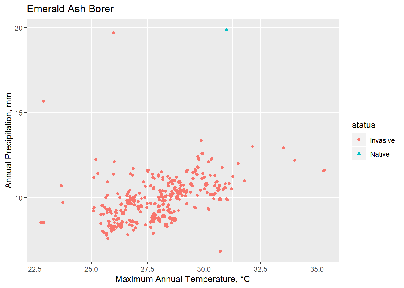
Emerald Ash Borer, Agrilus planipennis
#####Extracting Environmental Space per Species#####

#Emerald Ash Borer
EABsp<-SpatialPoints(cbind(EABdf$longitude, EABdf$latitude))
EABprec<-raster::extract(prec_annual, EABsp, fun=max, na.rm=TRUE, small=TRUE, sp=TRUE)%>%
  st_as_sf()

EABtmax<-raster::extract(tmax_annual, EABsp, fun=max, na.rm=TRUE, small=TRUE, sp=TRUE)%>%
  st_as_sf()

EABUSclim<-st_join(EABprec, EABtmax)%>%
  mutate(status="Invasive")

EABnsp<-SpatialPoints(cbind(EABndf$longitude, EABndf$latitude))
EABntmax<-raster::extract(tmax_annual, EABnsp, fun=max, na.rm=TRUE, small=TRUE, sp=TRUE)%>%
  st_as_sf()
EABnprec<-raster::extract(prec_annual, EABnsp, fun=max, na.rm=TRUE, small=TRUE, sp=TRUE)%>%
  st_as_sf()

EABnUSclim<-st_join(EABnprec,EABntmax)%>%
  mutate(status="Native")

EABmaster<-rbind(EABnUSclim, EABUSclim)
Spotted Lanternfly, Lycorma delicutula
SLFsp<-SpatialPoints(cbind(SLFdf$longitude, SLFdf$latitude))
SLFprec<-raster::extract(prec_annual, SLFsp, fun=max, na.rm=TRUE, small=TRUE, sp=TRUE)%>%
  st_as_sf()

SLFtmax<-raster::extract(tmax_annual, SLFsp, fun=max, na.rm=TRUE, small=TRUE, sp=TRUE)%>%
  st_as_sf()

SLFUSclim<-st_join(SLFprec, SLFtmax)%>%
  mutate(status="Invasive")

SLFnsp<-SpatialPoints(cbind(SLFndf$longitude, SLFndf$latitude))
SLFntmax<-raster::extract(tmax_annual, SLFnsp, fun=max, na.rm=TRUE, small=TRUE, sp=TRUE)%>%
  st_as_sf()
SLFnprec<-raster::extract(prec_annual, SLFnsp, fun=max, na.rm=TRUE, small=TRUE, sp=TRUE)%>%
  st_as_sf()

SLFnUSclim<-st_join(SLFnprec,SLFntmax)%>%
  mutate(status="Native")

SLFmaster<-rbind(SLFnUSclim, SLFUSclim)
Hemlock Woolly Adelgid, Adelges tsugae
HWAsp<-SpatialPoints(cbind(HWAdf$longitude, HWAdf$latitude))
HWAprec<-raster::extract(prec_annual, HWAsp, fun=max, na.rm=TRUE, small=TRUE, sp=TRUE)%>%
  st_as_sf()

HWAtmax<-raster::extract(tmax_annual, HWAsp, fun=max, na.rm=TRUE, small=TRUE, sp=TRUE)%>%
  st_as_sf()

HWAUSclim<-st_join(HWAprec, HWAtmax)%>%
  mutate(status="Invasive")

HWAnsp<-SpatialPoints(cbind(HWAndf$longitude, HWAndf$latitude))
HWAntmax<-raster::extract(tmax_annual, HWAnsp, fun=max, na.rm=TRUE, small=TRUE, sp=TRUE)%>%
  st_as_sf()
HWAnprec<-raster::extract(prec_annual, HWAnsp, fun=max, na.rm=TRUE, small=TRUE, sp=TRUE)%>%
  st_as_sf()

HWAnUSclim<-st_join(HWAnprec,HWAntmax)%>%
  mutate(status="Native")

HWAmaster<-rbind(HWAnUSclim, HWAUSclim)
Asian Long-horned Beetle, Anoplophora glabripennis
ALBsp<-SpatialPoints(cbind(ALBdf$longitude, ALBdf$latitude))
ALBprec<-raster::extract(prec_annual, ALBsp, fun=max, na.rm=TRUE, small=TRUE, sp=TRUE)%>%
  st_as_sf()

ALBtmax<-raster::extract(tmax_annual, ALBsp, fun=max, na.rm=TRUE, small=TRUE, sp=TRUE)%>%
  st_as_sf()

ALBUSclim<-st_join(ALBprec, ALBtmax)%>%
  mutate(status="Invasive")

ALBnsp<-SpatialPoints(cbind(ALBndf$longitude, ALBndf$latitude))
ALBntmax<-raster::extract(tmax_annual, ALBnsp, fun=max, na.rm=TRUE, small=TRUE, sp=TRUE)%>%
  st_as_sf()
ALBnprec<-raster::extract(prec_annual, ALBnsp, fun=max, na.rm=TRUE, small=TRUE, sp=TRUE)%>%
  st_as_sf()

ALBnUSclim<-st_join(ALBnprec,ALBntmax)%>%
  mutate(status="Native")

ALBmaster<-rbind(ALBnUSclim, ALBUSclim)
Sirex Woodwasp, Sirex noctilio
SWWsp<-SpatialPoints(cbind(SWWdf$longitude, SWWdf$latitude))
SWWprec<-raster::extract(prec_annual, SWWsp, fun=max, na.rm=TRUE, small=TRUE, sp=TRUE)%>%
  st_as_sf()

SWWtmax<-raster::extract(tmax_annual, SWWsp, fun=max, na.rm=TRUE, small=TRUE, sp=TRUE)%>%
  st_as_sf()

SWWUSclim<-st_join(SWWprec, SWWtmax)%>%
  mutate(status="Invasive")

SWWnsp<-SpatialPoints(cbind(SWWndf$longitude, SWWndf$latitude))
SWWntmax<-raster::extract(tmax_annual, SWWnsp, fun=max, na.rm=TRUE, small=TRUE, sp=TRUE)%>%
  st_as_sf()
SWWnprec<-raster::extract(prec_annual, SWWnsp, fun=max, na.rm=TRUE, small=TRUE, sp=TRUE)%>%
  st_as_sf()

SWWnUSclim<-st_join(SWWnprec,SWWntmax)%>%
  mutate(status="Native")

SWWmaster<-rbind(SWWnUSclim, SWWUSclim)
Results
Interactive Leaflet Maps
Invasive Insect Occurrences in the United States
Invasive Insect Occurrences Outside of the United States
Plotting Environmental Space
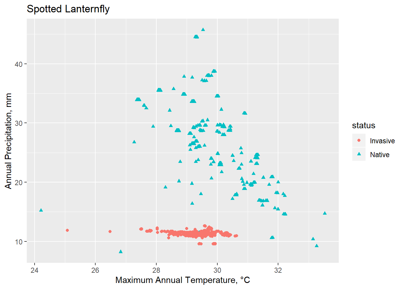
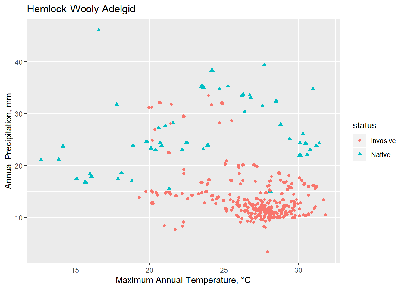
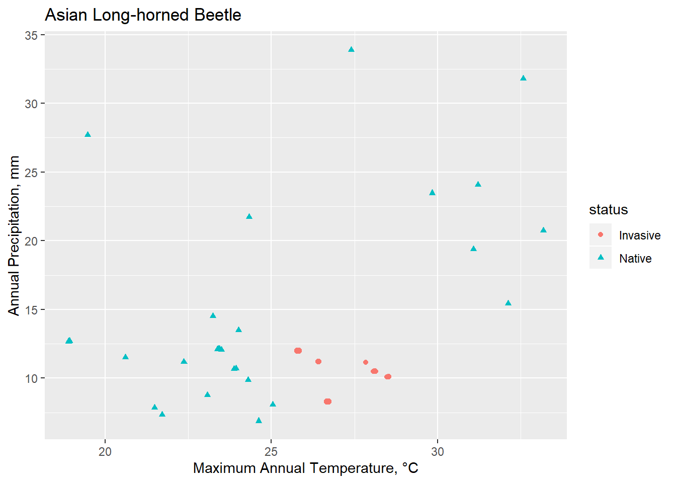
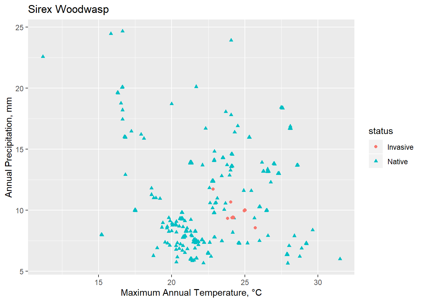
Conclusions
Though limited, Spocc is a useful tool for calling occurrence data. Invasion biology presents numerous challenges, in particular because an ecosystem currently under invasion is one that is not at equilibrium. Understanding how various environmental factors interact and create a habital and potentially vulnerable space to invasive species is an essential management strategy.
Future Directions
This approach becomes particularly important in the face of global climate change. Warming will likely facilitate the spread of invasive insects, and understanding these vulnerabilities is essential to preventative strategies
References
Evans, Alexander M. “Invasive Plants, Insects, and Diseases in the Forests of the Anthropocene.” Forest Conservation in the Anthropocene: Science, Policy, and Practice, edited by V. Alaric Sample et al., University Press of Colorado, Boulder, 2016, pp. 33–42. JSTOR, www.jstor.org/stable/j.ctt1f89r47.6.
Roderick, George, and Philippe Vernon “INVASION BIOLOGY.” Encyclopedia of Islands, edited by ROSEMARY G. GILLESPIE and DAVID A. CLAGUE, 1st ed., University of California Press, 2009, pp. 475–480. JSTOR, www.jstor.org/stable/10.1525/j.ctt1pn90r.110.