The Construction and Deconstruction of Empanada
Using lava flow morphology and mass wasting scars to determine if Empanada fell apart while it was being built
Katlyn Sewell
Introduction
Seamounts are oceanic volcanoes that form at nearly all seafloor tectonic settings. As oceanic plates are pulled apart, fissures form and eruptions of basaltic melt derived from decompression melting of the mantle occur. Over the course of hours to days, magmatic eruptions are focused in the center of the fissure because the thinner ends cool more rapidly. As the lava from this focused erutpion cools it builds the flanks of the seamount. Mass-wasting events are recorded in the morphology of seamounts as amphitheater shaped head scarps, talus, and erosive channels. Very few seamounts have been observed during construction, largely due to their remote location at the seafloor and difficulty detecting an erupting seamount from the surface. For these reasons much of their construction and deconstruction is based on scientific assumptions.
The Galapagos Spreading Center is a uniquely complex setting where the Nazca and Cocos plates meet within 100km of the Galapagos Hotspot. This study will look at the seamount Emapanada(2º6’N 92ºW) which is located on the Galapagos Spreading Center, off the coast of Ecuador. I hypothesis that Empanada experienced mass-wasting concurrent to its construction rather than exclusively after it. To test this hypothesis, I will look for changes in flank slope. The assessment will include a map of Empanada’s morphology based on previously collected dive video/pictures.
Ultimately, this project seeks to determine where Empanada has experienced mass-wasting.
Materials and Methods
- Load requied packages (you may need to install some of them)
library(plotly) #3d plot
library(raster) # package for raster manipulation
library(rgdal) # package for geospatial analysis
library(ggplot2) # package for plotting
library(data.table)
library(readxl) #read excel file
library(sf)
library(sp) #converting lat long to utm
library(rasterVis)
library(rio) #convert excel to csv
library(docxtractr) # reads .doc
library(tidyr) #used to split column into 2 columns
library(measurements) #convert deg min to decimal
library(jpeg) #read jpeg
library(dplyr) #mutate columnsGet the raster. The raster file used in this project used to be available online at http://www.soest.hawaii.edu/gruvee/sci/Alvin_Dives/gruvee-sentry-deployments.html; however, the website has broken and due to lack of interest the moderator, Scott White, has decided it’s not worth fixing. He is more than happy to send the data to any interested scientists upon email request. You may reach him at swhite@geol.sc.edu. For this reason, I have included the raster used in the data file rather than provide code to download it directly.
Open the raster file and assign it to an object. The z values are actually depths(distance below sea level) rather than elevation (distance above sea level) so we need to multiply the z values by -1 to plot accurately.
sm <- raster("data/empanada_clip.tif")*(-1)- Before we get too far it’s important to know what projection we need to use. Empanada is in UTM Zone 15N so we will assign it the proper projection.
proj="+proj=utm +zone=15 +ellps=GRS80 +datum=NAD83 +units=m +no_defs"
projection(sm)=proj- Download the port transcript for dive 4607 from the GRUVEE website. This excel sheet contains mass-wasting and lava morphology observations, as well as the X, Y positions where the observations were made.
dive_report <- "http://www.soest.hawaii.edu/gruvee/sci/Alvin_Dives/4607/Diver_Reports/4607_Port_transcript.xls"- Convert the .xls to .csv and read in the .csv
dive_report <- convert(dive_report, "dive_report.csv")
dive_4607 <- read.csv(dive_report)- The coordinates in the csv are a shorthand used by the GRUVEE crew rather than real coordinates. First we must calculate the conversion factor between the X, Y values and standard UTM.
#7a Download the sample collection file which contains X, Y and true coordinates from the GRUVEE website.
coordurl <- "http://www.soest.hawaii.edu/gruvee/sci/Alvin_Dives/4607/Diver_Reports/4607_Sample_table.doc"
coord <- read_docx(coordurl) #must have LibreOffice installed
#7b Now that you have a document with true coordinates and X, Y manually copy and paste the table into an excel file so you can work with it in R; I have included my ecxel file in the data folder. In this step, ensure that the table copied correctly and has the same number of rows and columns as the original.
#7c Read in the new excel file
coord_excel <- read_xlsx("data/coord_excel.xlsx")
#7d Seperate the latitude from the longitude
coord_split <- separate(coord_excel, "Lat, Long", c("Lat", "Long"), sep = "[,]")
#7e Convert the degree lat long into UTM. While I'm certain there is a way to do this in R, this programer was not able to discover it. Therefore, you must use an outside site to convert the degrees to UTM. I used this site: http://www.rcn.montana.edu/resources/converter.aspx
coord_split$Easting <- c(615760, 615809, 616218, 615848, 615918, 616063, 616180, 616302)
coord_split$Northing <- c(235171, 235154, 234317, 234133, 233736, 233416, 233151, 232770)
#7f Find the conversion factor to get from X to Easting and Y to Northing
## We know X + some# = Easting so Easting-X=conversion factor
coord_split[1, "Easting"] - coord_split[1, "X"]## Easting
## 1 600078## and Northing-Y=conversion factor
coord_split[1, "Northing"] - coord_split[1, "Y"]## Northing
## 1 224781## We can double check to make sure our conversion returns the correct values for all points
coord_split <- dplyr::mutate(coord_split, dbl_x= X + 600078)
coord_split <- dplyr::mutate(coord_split, dbl_y= Y + 224781)
dplyr::select(coord_split, Easting, Northing, dbl_x, dbl_y)## # A tibble: 8 x 4
## Easting Northing dbl_x dbl_y
## <dbl> <dbl> <dbl> <dbl>
## 1 615760 235171 615760 235171
## 2 615809 235154 615809 235154
## 3 616218 234317 616218 234318
## 4 615848 234133 615848 234133
## 5 615918 233736 615918 233736
## 6 616063 233416 615973 233416
## 7 616180 233151 616180 233151
## 8 616302 232770 616302 232770#Looks good! - Use the conversion factors to convert the X, Y positions from the dive 4607 transcript to standard UTM. A few aspects of our table need to be corrected before we can do this.
#8a. Correct the column names
names(dive_4607) <- lapply(dive_4607[8, ], as.character)
#8b. Remove the rows that do not contain observations
dive_4607 <- dive_4607[-c(1:8),]
#8c. Add a column name to the samples column
names(dive_4607)[7]<-"Samples"
#8d. Change the class of X and Y from factor to numeric
dive_4607[, "X"] <- as.numeric(as.character(dive_4607[, "X"]))
dive_4607[, "Y"] <- as.numeric(as.character(dive_4607[, "Y"] ))
#8e. Convert X and Y to accurate Easting and Northing as new columns
dive_4607 <- dplyr::mutate(dive_4607, Easting= X + 600078)
dive_4607 <- dplyr::mutate(dive_4607, Northing= Y + 224781)
#8f. Write this new table to a .csv file
write.csv(dive_4607, file = "data/dive_4607.csv") - Get the data ready to plot
dive_4607_sf <- read.csv("data/dive_4607.csv")%>% #read in the .csv file
drop_na(Easting) %>% #get rid of rows with NA values in the Easting column
st_as_sf(coords=c("Easting", "Northing")) %>% #set the coordinates
st_set_crs(proj) #set the projection
dive_crop <- st_crop(dive_4607_sf, xmin= 615000, xmax= 618000, ymin= 232000, ymax= 234000) #crop to show just the points over empanada- Plot the raster
emp1 <- gplot(sm) +
geom_tile(aes(fill=value))+
scale_fill_viridis_c()- Add the dive track to the 2D map
dive_track <- geom_sf(data=dive_crop, inherit.aes = F,col="red", size=0.5, mapping=aes())
emp2 <- emp1 + dive_track- Take a look
emp2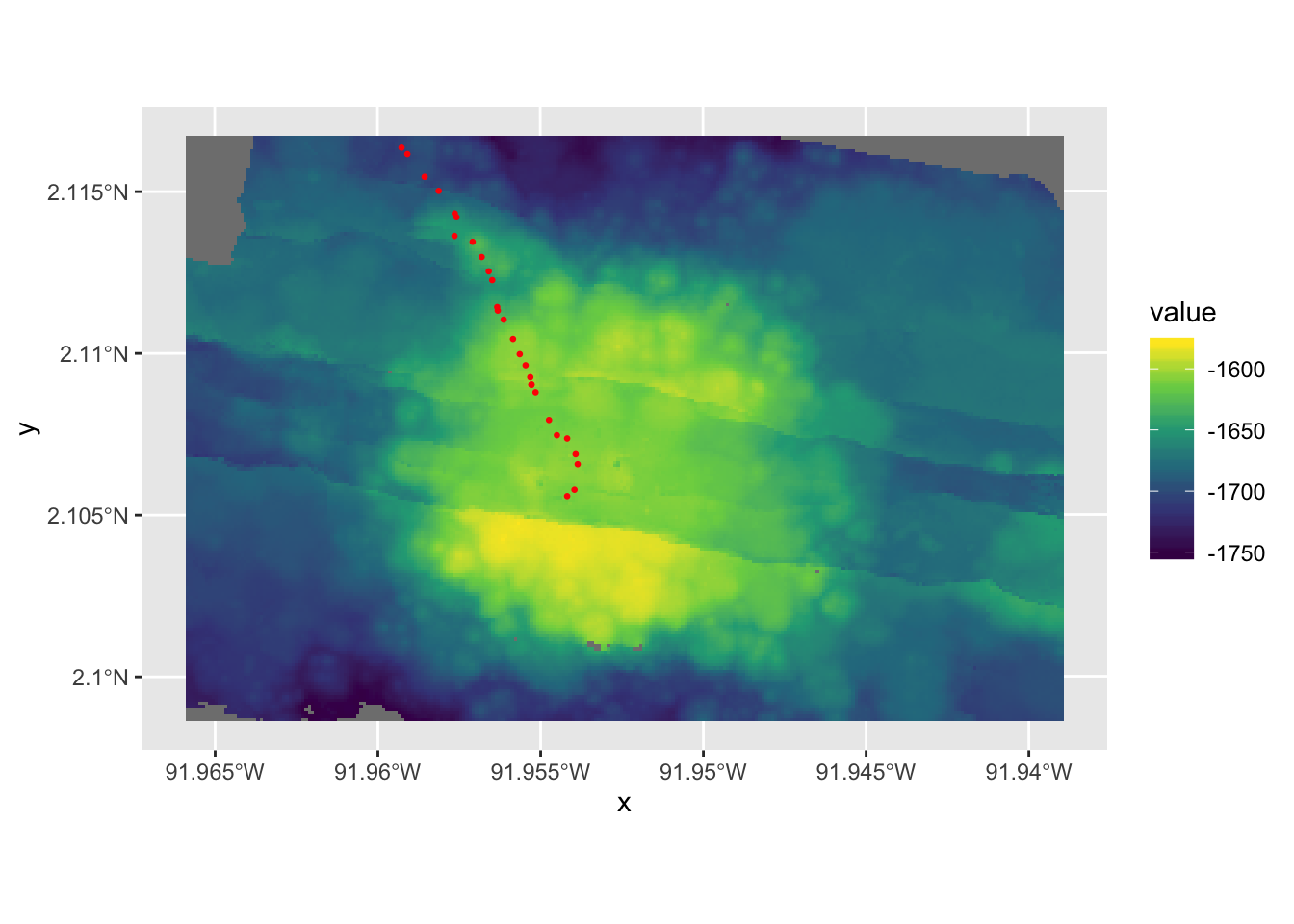
- To be sure our points are accurate we should refernce the dive map posted by the GRUVEE team
mapurl="http://www.soest.hawaii.edu/gruvee/sci/Alvin_Dives/4607/Diver_Reports/4607_Dive_map.jpg"
download.file(mapurl, 'dive_map.jpg', mode = 'wb')
plot_jpeg = function(path, add=FALSE) #referenced from stackexchange (see references)
{
require('jpeg')
jpg = readJPEG(path, native=T) # read the file
res = dim(jpg)[2:1] # get the resolution, [x, y]
if (!add) # initialize an empty plot area if add==FALSE
plot(1,1,xlim=c(1,res[1]),ylim=c(1,res[2]),asp=1,type='n',xaxs='i',yaxs='i',xaxt='n',yaxt='n',xlab='',ylab='',bty='n')
rasterImage(jpg,1,1,res[1],res[2])
}
plot_jpeg('dive_map.jpg')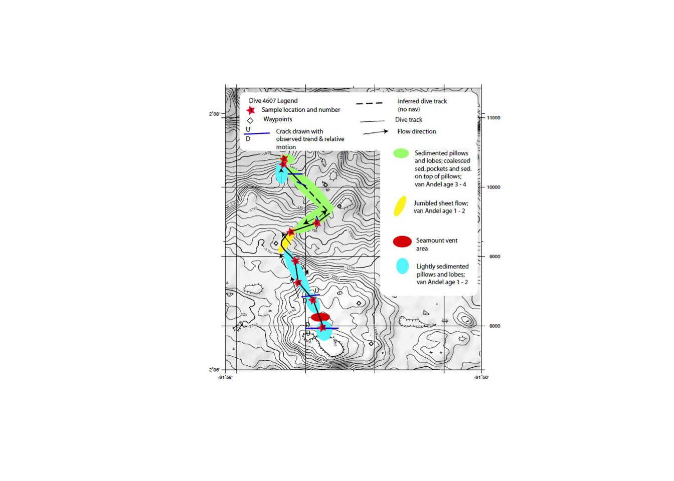
Our points look good!
Before we move on to the analysis let’s take a look at a 3-D plot of Empanada, just to get a good feel for what we’re working with.
sm_matrix <- as.matrix(sm)
plot_ly(z= ~sm_matrix, x=xFromCol(sm), y=yFromRow(sm)) %>%
add_surface() %>%
layout(scene= list(aspectmode='manual',
aspectratio = list(x=1, y=1, z=0.2)))